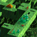
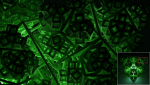
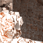
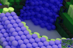
The king of the potato people does let me
2010-08-24 at 18:14 | Posted in Computer path | 1 CommentTags: 3D, art, C++, engine, fractal, maths, procedural, programming, pseudorandom, radiosity, random, ray tracing, raydiant, raytracing, realtime, render
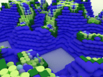
Firstly, this picture is an evolution of ‘The king of the potato people won’t let me’ (which you can see in the ‘Art’ tab of this blog). This new version has been rendered using the new Raydiant engine. It has much better quality (36 megapixel) so it can be printed at large sizes with high fidelity. This also allows for the potato people to be seen in better detail. And this is the kind of image that needs to be seen on big formats to be enjoyed. Has plenty of mysterious little ester eggs buried all along its green maze. The procedural generation of this image has led to the debugging of several pretty nasty and hard to find bugs on Raydiant, which is now more stable and also appreciably faster than before. May be I’ll post a real time interactive exploration demo for Linux (which is already working well in Raydiant). This picture has extended life time once printed, you can easily spend hours visually exploring its extremely detailed maze. Here are some zooms:


Custom probability distribution: fist of death update pack
2010-06-10 at 18:00 | Posted in Computer path | Leave a commentTags: 3D, art, C++, engine, fractal, maths, procedural, programming, pseudorandom, radiosity, random, ray tracing, raydiant, raytracing, realtime, render
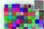
You probably remember that post where a symbolic way to obtain your pseudorandom number generator with custom probability distribution from a homogenous pseudorandom number generator (= a normal one like for example the standard C function rand()) was shown. Just in case it is here. That’s all good but it uses integrals. So now and then, depending on the custom probability distribution you want, it is not practical/possible to symbolically integrate the formula. For example for discontinuous probability distributions or something waving (like the image at the bottom) it may not work. What to do in those cases?. If you want it bad you can have it with some numeric integration. Basically you supply the code with your desired probability density function then the code does its magic and you can now get your crazily distributed pseudorandom numbers. All along this code ‘t’ is used to designate pseudorandom numbers with the custom probability density and ‘r’ pseudorandom numbers with nominal constant probability density of 1. I’ve extracted just the interesting parts from my tProbabilityDistributionCrusher class so object bureaucracy is lost in favour of clarity. Here is the initialization code full of useful annotations:
/**
 * this table is used to store values of:
 *    r = definite integral of E(x) between x=0 and x=t.
 *    (see 'Raydiant: custom probability distribution' post)
 * The first element holds the value of the integral for t
 * just greater than 0, the last element holds the
 * value of the integral for t just less than 1.
 * Any two consecutive elements have associated t values (not
 * stored) separated exactly by 1.0/areaFrom0ToEachT.count.
 */
 tArray *areaFrom0ToEachT;

 /** areaFrom0ToEachT.count */
 double realTableCount;

 /** inverse of areaFrom0ToEachT.count */
 double inverseTableCount;

/**
 * stepPrecisionCount is the number of steps used for numeric
 * integration, choose too few and that would give bad
 * quality, choose to many and accumulative errors may grow
 * high (but even for 10000000 they have been found to be
 * negligible).
 * Before compiling this function you must define your
 * custom probability function customProbabilityDensityFunction()
 * with anything you want
 */
void init(int integrationSteps)
{
   // misc initialization
   realTableCount = integrationSteps;
   inverseTableCount = double(1.0/realTableCount);
   // just use your favourite array class here:
   areaFrom0ToEachT = new tArray(integrationSteps);
   areaFrom0ToEachT->count = integrationSteps;

   // fill numeric definite integration table
   double area = 0;
   for(int i=1;i<=integrationSteps;++i)
   {
      double t = double(i)*inverseTableCount;// (0,1]
      assert(0.0<t && t<=1.0);
      double height = customProbabilityDensityFunction(t);
      assert(0<=height);
      area += inverseTableCount*height;
      (*areaFrom0ToEachT)[i-1] = area;
   }

   // lets normalize the area to 1.0
   double invArea = double(1.0/area);
   for(int i=0;i<integrationSteps;++i)
   {
      (*areaFrom0ToEachT)[i] *= invArea;
   }
 }
Here is an example definition of customProbabilityDensityFunction():
/**
 * this defines a waving probability distribution, t is
 * espected to be in the interval (0,1]
 */
double customProbabilityDensityFunction(const double& t)
{
   return 0.1+cos(20.0*t)+1.0;
}
And now this is how to obtain the pseudorandom numbers:
/**
 * returns a random number with the custom probability
 * density function
 */
double get_t()
{
   // get the nominal random number
   assert(areaFrom0ToEachT && int(realTableCount)==areaFrom0ToEachT->count);
   // rnd() must return a normal psudorandom number in the interval [0,1) :
   double r = rnd();

   // find where r is at our integration table, a plain binary search
   // is performed here and lower bound ndx returned:
   int ndx = areaFrom0ToEachT->getLowerBoundBinarySearch(r);

   // deal with extreme values
   if(ndx==areaFrom0ToEachT->count)
   {
      return 0.9999999999999;// just under 1.0
   }
   if(ndx==0)
   {
      return 0;
   }
   assert(0<ndx && ndxcount);

   // lets calc two bounding t values for that place at our
   // integration table
   double t0 = double(ndx)*inverseTableCount;
   assert(0.0<t0 && t0<1.0);
   double t1 = double(ndx+1)*inverseTableCount;
   assert(0.0<t1 && t1<=1.0);

   // lets find the master interpolation coefficient between the
   // two bounding t values
   double complementaryFractional01 =
      ((*areaFrom0ToEachT)[ndx]-r)
      /
      ((*areaFrom0ToEachT)[ndx]-(*areaFrom0ToEachT)[ndx-1]);
   assert(0.0<=complementaryFractional01 && complementaryFractional01<1.0);
   double interpolatedT =
      double(t0*complementaryFractional01+t1*(1.0-complementaryFractional01));
   assert(0.0<interpolatedT && interpolatedT<1.0);
   return interpolatedT;
}
With this code you could easily obtain probability distributions like this one:

Good luck and thanks for listening!
Intimacity, rare tracks
2010-06-08 at 17:11 | Posted in Computer path | Leave a commentTags: 3D, art, C++, engine, fractal, global illumination, maths, path tracing, procedural, programming, radiosity, ray tracing, raydiant, raytracing, realtime, render
Over a hundred renders of the Intimacity landscape have been performed till now. Two of them have made it to the final stage and won the price (the price meaning being rendered at HQ and published at deviant art here and here) and at least one more is following soon (waiting for a Zalman cooling device for my main PC and another i7 is coming so I can keep programming while rendering with it). But there are a few of the unselected renders that are still interesting. Thankyou all for the support!
![]()
Closer fold-the-bar-three-leaf-clover
2010-06-01 at 17:56 | Posted in Computer path | Leave a commentTags: 3D, art, C++, engine, fractal, maths, procedural, programming, radiosity, ray tracing, raydiant, raytracing, realtime, render
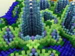
Here, some close up views of this HQ render. These zooms have still pretty good resolution. The Raydiant engine uses no short cuts with global illumination, all effort is put to optimize the real worse case scenario. Make sure to view the images full size.


The opposite river bank, zooms
2010-05-19 at 18:43 | Posted in Computer path | Leave a commentTags: 3D, art, C++, engine, fractal, global illumination, maths, path tracing, procedural, programming, radiosity, ray tracing, raydiant, raytracing, realtime, render
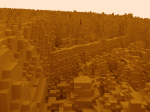
A new picture has been added to the collection at the art tab. Its name is ‘The opposite river bank’, depicts a copper veined marble landscape based on a variant of Alberto’s Maze function. These are some zoomed details of the high definition printable version here. The Raydiant engine has been used to render it. This particular view of the scenario was obtained during a real time full global illumination interactive walk.


Enmantled details
2010-05-15 at 11:06 | Posted in Computer path | Leave a commentTags: 3D, art, C++, engine, fractal, maths, procedural, programming, radiosity, ray tracing, raydiant, raytracing, realtime, render
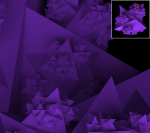
A new picture called ‘Enmantled’. Is formed using hiperdimensional versions of the Alberto’s Maze formula. The high resolution printed version os this new picture can be grasped better through these zooms. The complete picture is here and at the art tab of this blog.


Sweet gypsum flavour in detail
2010-05-09 at 17:23 | Posted in Computer path | Leave a commentTags: 3D, art, C++, engine, fractal, maths, procedural, programming, radiosity, ray tracing, raydiant, raytracing, realtime, render
Some zoomed details of the ‘Sweet gypsum flavour’ picture. The printable version has still more resolution. A classic backtracking algorithm with some custom tweaks was used to build the maze. Thanks to Maria for the image cooking.


Intimacity: the picture
2010-05-02 at 10:11 | Posted in Computer path | Leave a commentTags: 3D, art, C++, engine, fractal, global illumination, maths, path tracing, procedural, programming, radiosity, ray tracing, raydiant, raytracing, realtime, render
The definitive version of the Intimacity synthetic image is finalized. The printable one has 27 megapixel making for a very good definition on larger impressions (deviantart). My wife Maria has cooked some close ups to show several interesting details all over the city. I’ve spent hours looking around small areas of the landscape, the lighting varies subtlety allowing the pieces to have different appearances due to heterogeneous surrounding distributions. This scene has a complex global illumination equilibrium.


Blueberry hipersnowflake details
2010-05-01 at 13:16 | Posted in Computer path | Leave a commentTags: 3D, art, C++, engine, fractal, maths, procedural, programming, radiosity, ray tracing, raydiant, raytracing, realtime, render
A few zoomed details from the ‘blueberry hipersnowflake’ could be useful to assert the quality of the full resolution render. See it at deviantart. Thanks to my wife Maria for those images:

Intimacity lab tests
2010-04-22 at 16:39 | Posted in Computer path | Leave a commentTags: 3D, art, C++, engine, fractal, maths, procedural, programming, radiosity, ray tracing, raydiant, raytracing, realtime, render
I keep experimenting with Intimacity set. So many possibilities and so much fun. These are just a few samples. Also a coil of mirror spheres I found to be nice. It’s a big help to be able to walk in real time trough all this scenarios using the Raydiant engine then just take ‘photographs’ of the views you like. Furthermore, even I’m the one who built these scenario, it’s procedural so the exploration really satisfies my curiosity. The render speed of the Raydiant engine greatly facilitates the process.


- Computer path (rss) (58)
- September 2023 (1)
- July 2020 (1)
- August 2018 (1)
- September 2016 (1)
- December 2012 (1)
- October 2012 (1)
- January 2012 (1)
- December 2011 (1)
- September 2011 (1)
- August 2011 (1)
- April 2011 (1)
- March 2011 (1)
- February 2011 (1)
- January 2011 (1)
- September 2010 (2)
- August 2010 (1)
- June 2010 (3)
- May 2010 (5)
- April 2010 (3)
- February 2010 (1)
- January 2010 (1)
- December 2009 (1)
- November 2009 (23)
- October 2009 (4)
Categories:
Archives:
Blogroll
Blog at WordPress.com.
Entries and comments feeds.
